Autoencoders & Variational Autoencoders (VAE)
A plain autoencoder compresses then reconstructs. It memorizes. It does not generate. Add one trick, force the code to look Gaussian, and you get a sampler. That single trick, the reparameterization of $z = \mu + \sigma \cdot \epsilon$, is why every latent-diffusion and flow-matching image model you use in 2026 has a VAE at the input.
The Problem
Compress a 784-pixel MNIST digit to a 16-number code, then reconstruct. A plain autoencoder will ace reconstruction MSE but the code space is a lumpy mess. Pick a random point in the code space, decode it, and you get noise. It has no sampler. It is a compression model dressed up.
What you actually want is: (a) the code space is a clean, smooth distribution you can sample from, say an isotropic Gaussian $\mathcal{N}(0, I)$, (b) decoding any sample produces a plausible digit, and (c) the encoder and decoder still compress well. Three goals, one architecture, one loss.
Kingma's 2013 VAE solves this by training the encoder to output a distribution $q(z \mid x) = \mathcal{N}(\mu(x), \sigma(x)^2)$, pulling that distribution toward the prior $\mathcal{N}(0, I)$ via a KL penalty, and then sampling $z$ from $q(z \mid x)$ before decoding. At inference time, drop the encoder, sample $z \sim \mathcal{N}(0, I)$, decode. The KL penalty is what forces the code space to be structured.
In 2026 VAEs rarely ship standalone, they have been outclassed by diffusion for raw image quality, but they are the encoder of choice for every latent-diffusion model (SD 1/2/XL/3, Flux, AudioCraft). Learn the VAE and you learn the invisible first layer of every image pipeline you use.
The Concept
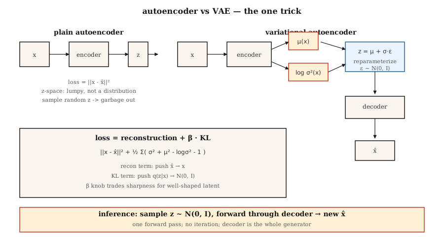
Autoencoder. $z = \text{encoder}(x)$, $\hat{x} = \text{decoder}(z)$, loss = $\lVert x - \hat{x} \rVert^2$. Code space unstructured.
VAE encoder. Outputs two vectors: $\mu(x)$ and $\log \sigma^2(x)$. These define $q(z \mid x) = \mathcal{N}(\mu, \mathop{\mathrm{diag}}(\sigma^2))$.
Reparameterization trick. Sampling from $q(z \mid x)$ is not differentiable. Rewrite the sample as $z = \mu + \sigma \cdot \epsilon$ where $\epsilon \sim \mathcal{N}(0, I)$. Now $z$ is a deterministic function of $(\mu, \sigma)$ plus a non-parameter noise, gradients flow through μ and $\sigma$.
Loss. Evidence Lower BOund (ELBO), two terms:
Reconstruction pushes $\hat{x}$ toward $x$. KL pushes $q(z \mid x)$ toward the prior. They trade off. Small $\beta$ ($<1$) = sharper samples, code space less Gaussian. Large $\beta$ ($>1$) = cleaner code space, blurrier samples. β-VAE (Higgins 2017) made this knob famous and kicked off disentanglement research.
Sampling. At inference: draw $z \sim \mathcal{N}(0, I)$, forward through decoder. One forward pass, no iterative sampling like diffusion.
Build It
code/main.py implements a tiny VAE without numpy or torch. Input is 8-dimensional synthetic data drawn from a 2-component Gaussian mixture in 8-D. Encoder and decoder are single hidden-layer MLPs. We implement tanh activation, forward pass, loss, and a hand-written backward pass. Not production, pedagogy.
Step 1: encoder forward
def encode(x, enc):
    h = tanh(add(matmul(enc["W1"], x), enc["b1"]))
    mu = add(matmul(enc["W_mu"], h), enc["b_mu"])
    log_sigma2 = add(matmul(enc["W_sig"], h), enc["b_sig"])
    return mu, log_sigma2
$\log \sigma^2$ instead of $\sigma$ so the network output is unconstrained (softplus of σ is a trap, gradients die at $\sigma \approx 0$).
Step 2: reparameterize and decode
def reparameterize(mu, log_sigma2, rng):
    eps = [rng.gauss(0, 1) for _ in mu]
    sigma = [math.exp(0.5 * lv) for lv in log_sigma2]
    return [m + s * e for m, s, e in zip(mu, sigma, eps)]

def decode(z, dec):
    h = tanh(add(matmul(dec["W1"], z), dec["b1"]))
    return add(matmul(dec["W_out"], h), dec["b_out"])
Step 3: the ELBO
def elbo(x, x_hat, mu, log_sigma2, beta=1.0):
    recon = sum((a - b) ** 2 for a, b in zip(x, x_hat))
    kl = 0.5 * sum(math.exp(lv) + m * m - lv - 1 for m, lv in zip(mu, log_sigma2))
    return recon + beta * kl, recon, kl
Exact closed-form KL because both distributions are Gaussian. Do not integrate numerically. People still ship code with monte-carlo KL estimates in 2026, it is 3x slower for no reason.
Step 4: generate
def sample(dec, z_dim, rng):
    z = [rng.gauss(0, 1) for _ in range(z_dim)]
    return decode(z, dec)
That is the generative model. Five lines.
Pitfalls
- Posterior collapse. KL term drives $q(z \mid x) \to \mathcal{N}(0, I)$ so aggressively that $z$ carries no info about $x$. Fix: β-annealing (start $\beta=0$, ramp to 1), free bits, or skip the KL on inactive dimensions.
- Blurry samples. The Gaussian decoder likelihood implies MSE reconstruction, which is Bayes-optimal for L2 (the mean), the mean of a set of plausible digits is a fuzzy digit. Fix: discrete decoder (VQ-VAE, NVAE), or use the VAE only as an encoder and stack diffusion on the latents (this is what Stable Diffusion does).
- β too large, too early. See posterior collapse. Start at $\beta \approx 0.01$ and ramp.
- Latent dim too small. 16-D works for MNIST, 256-D for ImageNet 256², 2048-D for ImageNet 1024². Stable Diffusion's VAE compresses 512×512×3 → 64×64×4 (32x downsample factor in spatial area, 32x in channels).
Use It
The 2026 VAE stack:
| Situation | Pick |
|---|---|
| Image-latent encoder for diffusion | Stable Diffusion VAE (sd-vae-ft-ema) or Flux VAE |
| Audio-latent encoder | Encodec (Meta), SoundStream, or DAC (Descript) |
| Video latents | Sora's spatiotemporal patches, Latte VAE, WAN VAE |
| Disentangled representation learning | β-VAE, FactorVAE, TCVAE |
| Discrete latents (for transformer modelling) | VQ-VAE, RVQ (ResidualVQ) |
| Continuous latents for generation | Plain VAE, then condition a flow/diffusion model in that latent space |
A latent-diffusion model is a VAE with a diffusion model living between encoder and decoder. The VAE does coarse compression, the diffusion model does the heavy lifting. Same pattern for video (VAE + video-diffusion DiT) and audio (Encodec + MusicGen transformer).
Ship It
Save outputs/skill-vae-trainer.md.
Skill takes: dataset profile + latent-dim target + downstream use (reconstruction, sampling, or latent-diffusion input) and outputs: architecture choice (plain/β/VQ/RVQ), β schedule, latent dim, decoder likelihood (Gaussian vs categorical), and evaluation plan (recon MSE, KL per dim, Fréchet distance between $q(z \mid x)$ and $\mathcal{N}(0, I))$.
Exercises
- Easy. Change $\beta$ in
code/main.pyto0.010.11.05.0. Record the final reconstruction MSE and KL. Which $\beta$ is Pareto-best for your synthetic data? - Medium. Replace the Gaussian decoder likelihood with a Bernoulli likelihood (cross-entropy loss). Compare sample quality on a binarized version of the same synthetic data.
- Hard. Extend
code/main.pyinto a mini VQ-VAE: replace the continuous $z$ with a nearest-neighbour lookup in a codebook of K=32 entries. Compare reconstruction MSE and report how many codebook entries get used (codebook collapse is real).
Key Terms
| Term | What people say | What it actually means |
|---|---|---|
| Autoencoder | Encode-decode network | $x \to z \to \hat{x}$, learn MSE. Not generative. |
| VAE | AE with a sampler | Encoder outputs a distribution, KL penalty shapes code space. |
| ELBO | Evidence lower bound | $\log p(x) \ge \text{recon} - \mathrm{KL}[q(z \mid x) \Vert p(z)]$; tight when $q = p(z \mid x)$. |
| Reparameterization | $z = \mu + \sigma \cdot \epsilon$ | Rewrites stochastic node as deterministic + pure noise. Enables backprop through sampling. |
| Prior | $p(z)$ | Target distribution for the latent, typically $\mathcal{N}(0, I)$. |
| Posterior collapse | "KL term wins" | Encoder ignores $x$, outputs the prior; decoder must hallucinate. |
| β-VAE | Tunable KL weight | $\text{loss} = \text{recon} + \beta \cdot \mathrm{KL}$. Higher $\beta$ = more disentangled but blurrier. |
| VQ-VAE | Discrete latent | Replace continuous $z$ with nearest codebook vector; enables transformer modelling. |
Production note: the VAE is the hottest path in a diffusion server
In a Stable Diffusion / Flux / SD3 pipeline the VAE is called twice per request, once to encode (if doing img2img / inpainting) and once to decode. At 1024² the decoder pass is often the single largest activation-memory peak in the whole pipeline because it upsamples 128×128×16 latents back to 1024×1024×3. Two practical consequences:
- Slice or tile the decode.
diffusersexposespipe.vae.enable_slicing()andpipe.vae.enable_tiling(). Tiling trades a small seam artifact for $O(\text{tile}^2)$ memory instead of $O(H \cdot W)$. Essential for 1024²+ on consumer GPUs. - bf16 decoder, fp32 numerics for the final resize. The SD 1.x VAE was released in fp32 and silently produces NaNs when cast to fp16 at 1024²+. SDXL ships
madebyollin/sdxl-vae-fp16-fixalways prefer the fp16-fix variant or use bf16.
Further Reading
- Kingma & Welling (2013). Auto-Encoding Variational Bayesthe VAE paper.
- Higgins et al. (2017). β-VAE: Learning Basic Visual Concepts with a Constrained Variational Frameworkdisentangled β-VAE.
- van den Oord et al. (2017). Neural Discrete Representation LearningVQ-VAE.
- Vahdat & Kautz (2021). NVAE: A Deep Hierarchical Variational Autoencoderstate-of-the-art image VAE.
- Rombach et al. (2022). High-Resolution Image Synthesis with Latent Diffusion ModelsStable Diffusion; VAE as encoder.
- Défossez et al. (2022). High Fidelity Neural Audio CompressionEncodec, the audio VAE standard.
The full code
Every file for this lesson. Copy it, run it, then change it.
import math
import random


def matmul(W, x):
    return [sum(w * xi for w, xi in zip(row, x)) for row in W]


def add(a, b):
    return [x + y for x, y in zip(a, b)]


def tanh(v):
    return [math.tanh(x) for x in v]


def tanh_grad(h):
    return [1 - x * x for x in h]


def randn_matrix(rows, cols, rng, scale=0.2):
    return [[rng.gauss(0, scale) for _ in range(cols)] for _ in range(rows)]


def init_vae(in_dim, hidden, z_dim, rng):
    return {
        "enc": {
            "W1": randn_matrix(hidden, in_dim, rng),
            "b1": [0.0] * hidden,
            "W_mu": randn_matrix(z_dim, hidden, rng),
            "b_mu": [0.0] * z_dim,
            "W_sig": randn_matrix(z_dim, hidden, rng),
            "b_sig": [0.0] * z_dim,
        },
        "dec": {
            "W1": randn_matrix(hidden, z_dim, rng),
            "b1": [0.0] * hidden,
            "W_out": randn_matrix(in_dim, hidden, rng),
            "b_out": [0.0] * in_dim,
        },
    }


def clamp(v, lo, hi):
    return [max(lo, min(hi, x)) for x in v]


def forward(x, params, eps):
    """Forward pass with a fixed epsilon for the reparameterization."""
    enc, dec = params["enc"], params["dec"]
    h_enc = tanh(add(matmul(enc["W1"], x), enc["b1"]))
    mu = add(matmul(enc["W_mu"], h_enc), enc["b_mu"])
    log_sigma2 = clamp(add(matmul(enc["W_sig"], h_enc), enc["b_sig"]), -6, 6)
    sigma = [math.exp(0.5 * lv) for lv in log_sigma2]
    z = [m + s * e for m, s, e in zip(mu, sigma, eps)]
    h_dec = tanh(add(matmul(dec["W1"], z), dec["b1"]))
    x_hat = add(matmul(dec["W_out"], h_dec), dec["b_out"])
    return {
        "h_enc": h_enc, "mu": mu, "log_sigma2": log_sigma2,
        "sigma": sigma, "z": z, "h_dec": h_dec, "x_hat": x_hat,
    }


def loss_value(x, fwd, beta):
    recon = sum((a - b) ** 2 for a, b in zip(x, fwd["x_hat"]))
    kl = 0.5 * sum(math.exp(lv) + m * m - lv - 1
                   for m, lv in zip(fwd["mu"], fwd["log_sigma2"]))
    return recon + beta * kl, recon, kl


def backward(x, fwd, params, beta):
    """Hand-written backprop. Returns gradient dict matching params shape."""
    enc, dec = params["enc"], params["dec"]
    mu, log_sigma2, sigma = fwd["mu"], fwd["log_sigma2"], fwd["sigma"]
    z, h_dec, h_enc = fwd["z"], fwd["h_dec"], fwd["h_enc"]
    x_hat = fwd["x_hat"]

    grads = {"enc": {}, "dec": {}}

    # d recon / d x_hat = 2(x_hat - x)
    d_x_hat = [2 * (a - b) for a, b in zip(x_hat, x)]

    # decoder: x_hat = W_out @ h_dec + b_out
    grads["dec"]["b_out"] = d_x_hat[:]
    grads["dec"]["W_out"] = [[d * h for h in h_dec] for d in d_x_hat]

    # d loss / d h_dec = W_out^T @ d_x_hat
    d_h_dec = [sum(dec["W_out"][i][j] * d_x_hat[i] for i in range(len(d_x_hat)))
               for j in range(len(h_dec))]
    # through tanh
    d_pre_dec = [dg * g for dg, g in zip(d_h_dec, tanh_grad(h_dec))]
    grads["dec"]["b1"] = d_pre_dec[:]
    grads["dec"]["W1"] = [[d * zi for zi in z] for d in d_pre_dec]

    # d loss / d z = W1_dec^T @ d_pre_dec
    d_z = [sum(dec["W1"][i][j] * d_pre_dec[i] for i in range(len(d_pre_dec)))
           for j in range(len(z))]

    # reparameterization: z = mu + sigma * eps, sigma = exp(0.5 * log_sigma2)
    # d z / d mu = 1, d z / d log_sigma2 = 0.5 * sigma * eps
    d_mu_recon = d_z[:]
    eps_used = [(z[i] - mu[i]) / max(sigma[i], 1e-8) for i in range(len(z))]
    d_lv_recon = [0.5 * d_z[i] * sigma[i] * eps_used[i] for i in range(len(z))]

    # KL term: 0.5 * sum(exp(lv) + mu^2 - lv - 1)
    # d KL / d mu = mu ; d KL / d lv = 0.5 * (exp(lv) - 1)
    d_mu = [d_mu_recon[i] + beta * mu[i] for i in range(len(mu))]
    d_lv = [d_lv_recon[i] + beta * 0.5 * (math.exp(log_sigma2[i]) - 1)
            for i in range(len(mu))]

    grads["enc"]["b_mu"] = d_mu[:]
    grads["enc"]["W_mu"] = [[d * h for h in h_enc] for d in d_mu]
    grads["enc"]["b_sig"] = d_lv[:]
    grads["enc"]["W_sig"] = [[d * h for h in h_enc] for d in d_lv]

    # d loss / d h_enc from both mu and log_sigma2 paths
    d_h_enc = [0.0] * len(h_enc)
    for j in range(len(h_enc)):
        for i in range(len(d_mu)):
            d_h_enc[j] += enc["W_mu"][i][j] * d_mu[i]
            d_h_enc[j] += enc["W_sig"][i][j] * d_lv[i]
    d_pre_enc = [dg * g for dg, g in zip(d_h_enc, tanh_grad(h_enc))]
    grads["enc"]["b1"] = d_pre_enc[:]
    grads["enc"]["W1"] = [[d * xi for xi in x] for d in d_pre_enc]
    return grads


def apply_update(params, grads, lr):
    for part in ("enc", "dec"):
        for name, tensor in params[part].items():
            g = grads[part][name]
            if isinstance(tensor[0], list):
                for i, row in enumerate(tensor):
                    for j in range(len(row)):
                        row[j] -= lr * g[i][j]
            else:
                for i in range(len(tensor)):
                    tensor[i] -= lr * g[i]


def sample_mixture(n, d, rng):
    data = []
    for _ in range(n):
        if rng.random() < 0.5:
            center = [1.0] * (d // 2) + [-1.0] * (d - d // 2)
        else:
            center = [-1.0] * (d // 2) + [1.0] * (d - d // 2)
        data.append([c + rng.gauss(0, 0.2) for c in center])
    return data


def mean(xs):
    return sum(xs) / max(len(xs), 1)


def main():
    rng = random.Random(7)
    in_dim, hidden, z_dim = 8, 10, 2
    params = init_vae(in_dim, hidden, z_dim, rng)
    data = sample_mixture(60, in_dim, rng)

    beta = 0.2
    lr = 0.01
    print(f"=== training tiny VAE: {in_dim}-D input, {z_dim}-D latent, beta={beta} ===")
    for epoch in range(40):
        losses, recons, kls = [], [], []
        for x in data:
            eps = [rng.gauss(0, 1) for _ in range(z_dim)]
            fwd = forward(x, params, eps)
            total, recon, kl = loss_value(x, fwd, beta)
            grads = backward(x, fwd, params, beta)
            apply_update(params, grads, lr)
            losses.append(total); recons.append(recon); kls.append(kl)
        if (epoch + 1) % 5 == 0:
            print(f"epoch {epoch+1:2d}: loss {mean(losses):.3f}  recon {mean(recons):.3f}  KL {mean(kls):.3f}")

    print()
    print("=== reconstruction on held-out sample ===")
    x_test = sample_mixture(1, in_dim, rng)[0]
    eps = [0.0] * z_dim
    fwd = forward(x_test, params, eps)
    mse = sum((a - b) ** 2 for a, b in zip(x_test, fwd["x_hat"]))
    print("  x     =", [f"{v:+.2f}" for v in x_test])
    print("  x_hat =", [f"{v:+.2f}" for v in fwd["x_hat"]])
    print(f"  mse = {mse:.3f}")

    print()
    print("=== samples from N(0, I) through decoder ===")
    for _ in range(4):
        z = [rng.gauss(0, 1) for _ in range(z_dim)]
        h = tanh(add(matmul(params["dec"]["W1"], z), params["dec"]["b1"]))
        x_hat = add(matmul(params["dec"]["W_out"], h), params["dec"]["b_out"])
        print(f"  z={[f'{zi:+.2f}' for zi in z]}  ->  x_hat={[f'{v:+.2f}' for v in x_hat]}")

    print()
    print("takeaway: decoder turns N(0, I) samples into structured 8-D vectors")
    print("          that resemble the two-cluster training data.")


if __name__ == "__main__":
    main()