Policy Gradient, REINFORCE from Scratch
Stop estimating value. Parameterize the policy directly, compute the gradient of expected return, step uphill. Williams (1992) wrote it in one theorem. It is why PPO, GRPO, and every LLM RL loop exist.
The Problem
Q-learning and DQN parameterize the value function. You pick actions by argmax Q. That is fine for discrete actions and discrete states. It breaks when actions are continuous (which argmax over a 10-dimensional torque?) or when you want a stochastic policy (argmax is deterministic by construction).
Policy gradients parameterize the policy instead. $\pi_\theta(a \mid s)$ is a neural net that outputs a distribution over actions. Sample from it to act. Compute the gradient of expected return with respect to $\theta$. Step uphill. No argmax. No Bellman recursion. Just gradient ascent on $J(\theta) = \mathbb E_{\pi_\theta}[G]$.
The REINFORCE theorem (Williams 1992) tells you this gradient is computable: $\nabla J(\theta) = \mathbb E_\pi[ G \cdot \nabla_\theta \log \pi_\theta(a \mid s) ]$. Run an episode. Compute the return. Multiply by $\nabla \log \pi_\theta(a \mid s)$ at every step. Average. Gradient-ascent. Done.
Every LLM-RL algorithm in 2026, PPO, DPO, GRPO, is a refinement of REINFORCE. Understanding it in your fingers is the prerequisite for the rest of this phase, and for Phase 10 · 07 (RLHF implementation) and Phase 10 · 08 (DPO).
The Concept
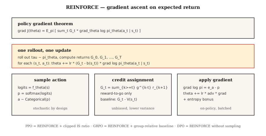
The policy gradient theorem. For any policy $\pi_\theta$ parameterized by $\theta$:
where $G_t = \sum_{k=t}^{T} \gamma^{k-t} r_{k+1}$ is the discounted return from step $t$. The expectation is over full trajectories $\tau$ sampled from $\pi_\theta$.
The proof is short. Differentiate $J(\theta) = \sum_\tau P(\tau; \theta) G(\tau)$ under the expectation. Use $\nabla P(\tau; \theta) = P(\tau; \theta) \nabla \log P(\tau; \theta)$ (the log-derivative trick). Factor $\log P(\tau; \theta) = \sum \log \pi_\theta(a_t \mid s_t) + \text{environment terms that do not depend on } \theta$. The environment terms vanish. Two lines of algebra give you the theorem.
Variance reduction tricks. Vanilla REINFORCE has murderous variance, returns are noisy, $\nabla \log \pi$ is noisy, their product is very noisy. Two standard fixes:
- Baseline subtraction. Replace $G_t$ with $G_t - b(s_t)$ for any baseline $b(s_t)$ that does not depend on $a_t$. Unbiased because $\mathbb{E}[b(s_t) \cdot \nabla \log \pi(a_t \mid s_t)] = 0$. Typical choice: $b(s_t) = \hat{V}(s_t)$ learned by a critic → actor-critic (Lesson 07).
- Reward-to-go. Replace $\sum_t G_t \cdot \nabla \log \pi_\theta(a_t \mid s_t)$ with $\sum_t G_t^{\text{from } t} \cdot \nabla \log \pi_\theta(a_t \mid s_t)$. Only future returns matter for a given action, past rewards contribute zero-mean noise.
Combined, you get:
which is REINFORCE with a baseline, the direct ancestor of A2C (Lesson 07) and PPO (Lesson 08).
Softmax policy parameterization. For discrete actions, the standard choice:
where $f_\theta$ is any neural net that outputs a score per action. The gradient has a clean form:
i.e., score of the taken action minus its expected value under the policy.
Gaussian policy for continuous actions. $\pi_\theta(a \mid s) = N(\mu_\theta(s), \sigma_\theta(s))$. $\nabla \log N(a; \mu, \sigma)$ has a closed form. That is all Phase 9 · 07's SAC needs.
Build It
Step 1: softmax policy network
def policy_logits(theta, state_features):
    return [dot(theta[a], state_features) for a in range(N_ACTIONS)]

def softmax(logits):
    m = max(logits)
    exps = [exp(l - m) for l in logits]
    Z = sum(exps)
    return [e / Z for e in exps]
Use a linear policy (one weight vector per action) for a tabular env. For Atari, swap in a CNN and keep the softmax head.
Step 2: sampling and log-probability
def sample_action(probs, rng):
    x = rng.random()
    cum = 0
    for a, p in enumerate(probs):
        cum += p
        if x <= cum:
            return a
    return len(probs) - 1

def log_prob(probs, a):
    return log(probs[a] + 1e-12)
Step 3: rollout with log-probs captured
def rollout(theta, env, rng, gamma):
    trajectory = []
    s = env.reset()
    while not done:
        logits = policy_logits(theta, s)
        probs = softmax(logits)
        a = sample_action(probs, rng)
        s_next, r, done = env.step(s, a)
        trajectory.append((s, a, r, probs))
        s = s_next
    return trajectory
Step 4: REINFORCE update
def reinforce_step(theta, trajectory, gamma, lr, baseline=0.0):
    returns = compute_returns(trajectory, gamma)
    for (s, a, _, probs), G in zip(trajectory, returns):
        advantage = G - baseline
        grad_log_pi_a = [-p for p in probs]
        grad_log_pi_a[a] += 1.0
        for i in range(N_ACTIONS):
            for j in range(len(s)):
                theta[i][j] += lr * advantage * grad_log_pi_a[i] * s[j]
The gradient $\nabla \log \pi(a \mid s) = e_a - \pi(\cdot \mid s)$ (onehot of $a$ minus probabilities) is the heart of softmax policy gradients. Burn it into muscle memory.
Step 5: baselines
A running mean of $G$ over recent episodes is enough variance reduction to get a 4×4 GridWorld running; it takes ~500 episodes to converge. Upgrade the baseline to a learned $\hat{V}(s)$ and you get actor-critic.
Pitfalls
- Exploding gradients. Returns can be huge. Always normalize $G$ to
~N(0, 1)across the batch before multiplying by $\nabla \log \pi$. - Entropy collapse. The policy converges to a near-deterministic action too early, stops exploring, gets stuck. Fix: add entropy bonus $\beta \cdot H(\pi(\cdot \mid s))$ to the objective.
- High variance. Vanilla REINFORCE needs thousands of episodes. A critic baseline (Lesson 07) or TRPO/PPO's trust region (Lesson 08) is the standard fix.
- Sample inefficiency. On-policy means you throw away every transition after one update. Off-policy corrections via importance sampling bring back data, at the cost of variance (PPO's ratio is a clipped IS weight).
- Non-stationary gradients. The same gradient from 100 episodes ago uses old $\pi$. On-policy methods update every few rollouts for this reason.
- Credit assignment. Without reward-to-go, past rewards contribute noise. Always use reward-to-go.
Use It
In 2026, REINFORCE is rarely run directly but its gradient formula is everywhere:
| Use case | Derived method |
|---|---|
| Continuous control | PPO / SAC with Gaussian policy |
| LLM RLHF | PPO with KL penalty, running on token-level policy |
| LLM reasoning (DeepSeek) | GRPO, REINFORCE with group-relative baseline, no critic |
| Multi-agent | Centralized-critic REINFORCE (MADDPG, COMA) |
| Discrete action robotics | A2C, A3C, PPO |
| Preference-only settings | DPO, REINFORCE rewritten as a preference-likelihood loss, no sampling |
When you read loss = -advantage * log_prob in a 2026 training script, that is REINFORCE with a baseline. Entire papers (DPO, GRPO, RLOO) are variance-reduction tricks on top of this one line.
Ship It
Save as outputs/skill-policy-gradient-trainer.md:
---
name: policy-gradient-trainer
description: Produce a REINFORCE / actor-critic / PPO training config for a given task and diagnose variance issues.
version: 1.0.0
phase: 9
lesson: 6
tags: [rl, policy-gradient, reinforce]
---

Given an environment (discrete / continuous actions, horizon, reward stats), output:

1. Policy head. Softmax (discrete) or Gaussian (continuous) with parameter counts.
2. Baseline. None (vanilla), running mean, learned `V̂(s)`, or A2C critic.
3. Variance controls. Reward-to-go on by default, return normalization, gradient clip value.
4. Entropy bonus. Coefficient β and decay schedule.
5. Batch size. Episodes per update; on-policy data freshness contract.

Refuse REINFORCE-no-baseline on horizons > 500 steps. Refuse continuous-action control with a softmax head. Flag any run with `β = 0` and observed policy entropy < 0.1 as entropy-collapsed.
Exercises
- Easy. Implement REINFORCE on 4×4 GridWorld with a linear softmax policy. Train for 1,000 episodes without a baseline. Plot the learning curve; measure variance (std of returns).
- Medium. Add a running-mean baseline. Train again. Compare sample efficiency and variance to the vanilla run. By how much does the baseline reduce steps to convergence?
- Hard. Add an entropy bonus $\beta \cdot H(\pi)$. Sweep $\beta \in \lbrace 0, 0.01, 0.1, 1.0 \rbrace$. Plot final return and policy entropy. Where is the sweet spot on this task?
Key Terms
| Term | What people say | What it actually means |
|---|---|---|
| Policy gradient | "Train the policy directly" | $\nabla J(\theta) = \mathbb{E}[G \cdot \nabla \log \pi_\theta(a \mid s)]$; derived from the log-derivative trick. |
| REINFORCE | "The original PG algorithm" | Williams (1992); Monte Carlo returns multiplied by log-policy gradient. |
| Log-derivative trick | "Score function estimator" | $\nabla P(\tau;\theta) = P(\tau;\theta) \cdot \nabla \log P(\tau;\theta)$; makes gradients of expectations tractable. |
| Baseline | "Variance reduction" | Any $b(s)$ subtracted from $G$; unbiased because $\mathbb{E}[b \cdot \nabla \log \pi] = 0$. |
| Reward-to-go | "Only future returns count" | $G_t^{\text{from } t}$ instead of the full $G_0$; correct and lower-variance. |
| Entropy bonus | "Encourage exploration" | $+\beta \cdot H(\pi(\cdot \mid s))$ term keeps the policy from collapsing. |
| On-policy | "Train on what you just saw" | Gradient expectation is w.r.t. the current policy, cannot reuse old data directly. |
| Advantage | "How much better than average" | $A(s, a) = G(s, a) - V(s)$; the signed quantity REINFORCE-with-baseline multiplies. |
Further Reading
- Williams (1992). Simple Statistical Gradient-Following Algorithms for Connectionist Reinforcement Learningthe original REINFORCE paper.
- Sutton et al. (2000). Policy Gradient Methods for Reinforcement Learning with Function Approximationthe modern policy-gradient theorem with function approximation.
- Sutton & Barto (2018). Ch. 13, Policy Gradient Methodstextbook presentation.
- OpenAI Spinning Up, VPG / REINFORCEclear pedagogical exposition with PyTorch code.
- Peters & Schaal (2008). Reinforcement Learning of Motor Skills with Policy Gradientsvariance-reduction and the natural-gradient view that connects REINFORCE to the trust-region family (TRPO, PPO).
The full code
Every file for this lesson. Copy it, run it, then change it.
import math
import random


GRID = 4
TERMINAL = (3, 3)
ACTIONS = ("up", "down", "left", "right")
DELTAS = {"up": (-1, 0), "down": (1, 0), "left": (0, -1), "right": (0, 1)}
N_ACTIONS = len(ACTIONS)
N_FEAT = GRID * GRID


def reset():
    return (0, 0)


def step(state, action_idx):
    if state == TERMINAL:
        return state, 0.0, True
    dr, dc = DELTAS[ACTIONS[action_idx]]
    r, c = state
    nr = min(max(r + dr, 0), GRID - 1)
    nc = min(max(c + dc, 0), GRID - 1)
    return (nr, nc), -1.0, (nr, nc) == TERMINAL


def features(state):
    x = [0.0] * N_FEAT
    r, c = state
    x[r * GRID + c] = 1.0
    return x


def init_theta(rng):
    return [[rng.gauss(0, 0.1) for _ in range(N_FEAT)] for _ in range(N_ACTIONS)]


def logits(theta, x):
    return [sum(w * xi for w, xi in zip(theta[a], x)) for a in range(N_ACTIONS)]


def softmax(z):
    m = max(z)
    exps = [math.exp(zi - m) for zi in z]
    Z = sum(exps)
    return [e / Z for e in exps]


def sample(probs, rng):
    x = rng.random()
    cum = 0.0
    for a, p in enumerate(probs):
        cum += p
        if x <= cum:
            return a
    return N_ACTIONS - 1


def rollout(theta, rng, max_steps=100):
    traj = []
    s = reset()
    for _ in range(max_steps):
        x = features(s)
        probs = softmax(logits(theta, x))
        a = sample(probs, rng)
        s_next, r, done = step(s, a)
        traj.append((x, a, r, probs))
        if done:
            break
        s = s_next
    return traj


def returns_to_go(traj, gamma):
    G = 0.0
    out = []
    for _, _, r, _ in reversed(traj):
        G = r + gamma * G
        out.append(G)
    out.reverse()
    return out


def reinforce(episodes, lr=0.05, gamma=0.99, use_baseline=False, rng=None):
    rng = rng or random.Random(0)
    theta = init_theta(rng)
    baseline = 0.0
    returns_log = []
    for ep in range(episodes):
        traj = rollout(theta, rng)
        returns = returns_to_go(traj, gamma)
        if use_baseline:
            baseline = 0.95 * baseline + 0.05 * returns[0]
        for (x, a, _r, probs), G in zip(traj, returns):
            adv = G - (baseline if use_baseline else 0.0)
            for i in range(N_ACTIONS):
                grad = (1.0 if i == a else 0.0) - probs[i]
                for j in range(N_FEAT):
                    theta[i][j] += lr * adv * grad * x[j]
        returns_log.append(returns[0] if returns else 0.0)
    return theta, returns_log


def greedy_policy(theta):
    policy = {}
    for r in range(GRID):
        for c in range(GRID):
            if (r, c) == TERMINAL:
                continue
            z = logits(theta, features((r, c)))
            policy[(r, c)] = ACTIONS[max(range(N_ACTIONS), key=lambda i: z[i])]
    return policy


def print_policy(policy, title):
    arrows = {"up": "^", "down": "v", "left": "<", "right": ">"}
    print(f"  {title}")
    for r in range(GRID):
        row = []
        for c in range(GRID):
            if (r, c) == TERMINAL:
                row.append(".")
            elif (r, c) in policy:
                row.append(arrows[policy[(r, c)]])
            else:
                row.append("?")
        print("   " + " ".join(row))


def block_mean(xs, block):
    return [sum(xs[i : i + block]) / block for i in range(0, len(xs) - block + 1, block)]


def main():
    episodes = 2000
    rng = random.Random(42)
    _, r_plain = reinforce(episodes, use_baseline=False, rng=rng)
    rng = random.Random(42)
    theta_b, r_base = reinforce(episodes, use_baseline=True, rng=rng)

    print(f"=== REINFORCE on 4x4 GridWorld, {episodes} episodes, lr=0.05, gamma=0.99 ===")
    print()
    print("learning curves (mean return per 200 episodes):")
    for i, (a, b) in enumerate(zip(block_mean(r_plain, 200), block_mean(r_base, 200))):
        print(f"  block {i+1}: vanilla={a:7.2f}   with-baseline={b:7.2f}")

    print()
    print_policy(greedy_policy(theta_b), "final greedy policy (with-baseline)")
    print()
    print(f"final mean return (last 200 eps): vanilla={sum(r_plain[-200:])/200:.2f}   with-baseline={sum(r_base[-200:])/200:.2f}")
    print("(optimal return on this 4x4 GridWorld = -6.0)")


if __name__ == "__main__":
    main()
Most people stop here. Don't be most people.
The next 6 lessons are where Phase 09 turns from understanding into ability: the harder builds, the production patterns and the quizzes that prove you've actually got it. Unlock the full AI Expert Masterclass: all 542 expert lessons, every line of code, every phase.
- 07Actor-Critic, A2C and A3C
- 08Proximal Policy Optimization (PPO)
- 09Reward Modeling & RLHF
- 10Multi-Agent RL
- + 2 more in this phase, and 542 across the whole masterclass